Good Times
by James Classen
The BBC has done it again. Sherlock is the best modern day Sherlock Holmes story, Benedict Cumberbatch the best Holmes since Jeremy Brett. Affectations, mannerisms, they’re “spot on.” I would very much suspect that the greatest consulting detective of all time would do much the same as this one, given today’s technology. I’ve only seen “A Study In Pink” and “The Blind Banker” so far, and while they’ve done the sensational stories first, I hope they delve deeper into development of the characters as the series progresses. It’s been too long since I’ve read the books, but I recognized so much of these episodes, and they remind me of “A Study In Scarlet” (obviously), “The Sign of the Four”, and “The Five Orange Pips” along with a hint of “The Adventure of the Dancing Men”. Had her name been Mary Morstan…but perhaps she’ll show up later.
The discrete Fourier transform. Simple enough, sure:

I have no problems with this. Or the conversion to a matrix formula:

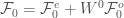
where 

Eventually I found the Danielson-Lanczos lemma, which gives

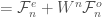
This is all fine and good. Then it comes to working the FFT, using the Danielson-Lanczos lemma and the Cooley-Tukey algorithm, I’m suddenly stumped. Not the mechanics, but the programming bit. I know I’ve done this successfully before, certainly in college and at least once since then—I had a Python script that used this, first to compute DFTs, then to multiply numbers. Obviously unnecessary with Python supporting arbitrary precision arithmetic built in, but the purpose was (and is) to bolster my own understanding of one of the principles behind APM.
So, University at Buffalo to the rescue. Found some C++ code that gave me what I needed. So here’s (hopefully) a more-or-less plain English version of the method (with an example):
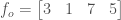
Given a vector (we’ll start small, a size of 8) 
If the number of elements in the vector is even, split the odd and even parts of the vector into separate vectors (so I cheated and chose a nice number. But the method doesn’t help if the above isn’t true). We’ll call those 


These are still divisible by two, so repeat:


Still even!


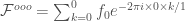
Now the size of these vectors is odd, so the only choice is to do a regular discrete transform. But this turns out to be nice and simple. Using superscripts to denote which of the above vectors I’m refering to, since

we can plug in each of the above into this formula:
which nicely reduces to

But this is only the discrete transform of the one-element vector—these need to be recombined to get the DFT of the entire thing.
So if you reduce the vectors to size 1, the DFT of that is trivial. Then we need to combine them. So let’s start that combination one level higher, with the two-element vectors.
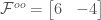
From the Danielson-Lanczos lemma,

Therefore,


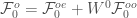
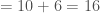
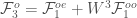
In this case, 

So for a two-element vector,

“Solving” the others in a similar manner, we get


Of course, each step gets a bit more difficult. Thanks to the DLL, we know

so let’s take it one step at a time.
First,

So


Therefore,

Do the same thing to find 

Putting it all together,


Thus

Seems like a lot of work, I know. But here’s the thing: normally, using the straight definition, you’d be doing 64 multiplications, 64 sums, and 64 exponentiations (


Yes, it’s still a lot of work, but as the vectors get longer, these savings adds up fast:
| Vector Size | Naive Operations | FFT operations |
|---|---|---|
| 1 | 1 | 0 |
| 2 | 4 | 2 |
| 4 | 16 | 8 |
| 8 | 64 | 24 |
| 16 | 256 | 64 |
| 32 | 1024 | 160 |
And once you put it in a computer program (like the following listing), massive data sets become easy to analyze.
